Next: Bibliography Up: True Path Rule hierarchical Previous: Classification of specific FunCat
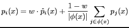
Fig. 7 and 8 show the hierarchical precision, recall and F-measure as functions of the parameter ![]() .
For small values of
.
For small values of ![]() (
(![]() can vary from 0 to 1) the weight of the decision of the parent local predictor is small, and the ensemble decision
depends mainly by the positive predictions of the offsprings nodes(classifiers): in this case we obtain a higher hierarchical recall for the TPR-w ensemble.
On the contrary higher values of
can vary from 0 to 1) the weight of the decision of the parent local predictor is small, and the ensemble decision
depends mainly by the positive predictions of the offsprings nodes(classifiers): in this case we obtain a higher hierarchical recall for the TPR-w ensemble.
On the contrary higher values of ![]() correspond to a higher weight of the ``parent'' local predictor, with a resulting higher precision.
The opposite trends of precision and recall are quite clear in all graphs of Fig. 7. The best F-score is in ``middle'' values
of the parameter parent-weight: in practice in most of the analyzed data sets the best F-measure is achieved for
correspond to a higher weight of the ``parent'' local predictor, with a resulting higher precision.
The opposite trends of precision and recall are quite clear in all graphs of Fig. 7. The best F-score is in ``middle'' values
of the parameter parent-weight: in practice in most of the analyzed data sets the best F-measure is achieved for ![]() between
between ![]() and
and ![]() , but if we need higher
recall rates (at the expense of the precision) we can choose lower
, but if we need higher
recall rates (at the expense of the precision) we can choose lower ![]() values, and higher values of
values, and higher values of ![]() are needed if precision is our first aim.
are needed if precision is our first aim.
|
|
![\includegraphics[width = 7.2cm]{eps/YeastDomainNobleBinary.c0.5.hier.2way.F.w.eps}](img12.png)
![\includegraphics[width = 7.2cm]{eps/YeastDomainNobleBinary.g0.001c100.hier.2way.F.w.eps}](img13.png)
![\includegraphics[width = 7.2cm]{eps/YeastBiogrid.c100.hier.2way.F.w.b0.eps}](img14.png)
![\includegraphics[width = 7.2cm]{eps/YeastBiogrid.g0.1c100.hier.2way.F.w.b0.eps}](img15.png)
![\includegraphics[width = 7.2cm]{eps/YeastVM.c1000.hier.2way.F.w.b0.eps}](img16.png)
![\includegraphics[width = 7.2cm]{eps/YeastVM.g0.1c100.hier.2way.F.w.b0.eps}](img17.png)
![\includegraphics[width = 7.2cm]{eps/YeastSW.c0.001.hier.2way.F.w.b0.eps}](img18.png)
![\includegraphics[width = 7.2cm]{eps/YeastSW.d3c1.hier.2way.F.w.eps}](img19.png)
![\includegraphics[width = 7.2cm]{eps/YeastDomainLog.c1000.hier.2way.F.w.b0.eps}](img20.png)
![\includegraphics[width = 7.2cm]{eps/YeastDomainLog.g1c100.hier.2way.F.w.b0.eps}](img21.png)
![\includegraphics[width = 7.2cm]{eps/Yeast.phylo.linear.F.w.b0.eps}](img22.png)
![\includegraphics[width = 7.2cm]{eps/Yeast.phylo.gauss.F.w.b0.eps}](img23.png)
![\includegraphics[width = 7.2cm]{eps/YeastExpr.c0.1.hier.2way.F.w.b0.eps}](img24.png)
![\includegraphics[width = 7.2cm]{eps/YeastExpr.g0.001c100.hier.2way.F.w.b0.eps}](img25.png)